Multithreaded Algorithms | Baeldung on Computer Science

1. Overview

In computer science, there are various parallel algorithms that can run on a multiprocessor computer, such as multithreaded algorithms.

In this tutorial, we’ll take a look at what this approach means. Then, we’ll use an example to understand it in a better way.

2. Concepts of Dynamic Multithreading

Multithreading is a crucial topic for modern computing. There exist many competing models of parallel computation that are essentially different. For example, one can have shared or distributed memory. Since multicore processors are ubiquitous, we focus on a parallel computing model with shared memory.

2.1. Dynamic and Static Multithreading

Static threading means that the programmer needs to specify how many processors to use at each point in advance. When it comes to evolving conditions, this can be inflexible.

In dynamic multithreading models, the programmer needs to specify opportunities for parallelism and a concurrency platform manages the decisions of mapping these opportunities to actual static threads.

2.2. Concurrency Constructs

A concurrency platform is a software layer that schedules, manages, and coordinates parallel-computing resources. We’ll use a simple extension of the serial programming model that reflects current parallel-computing practice:

Spawn: Instead of waiting for the child to finish, the procedure instance that executes the spawn (the parent) may continue to execute in parallel with the spawned subroutine (the child)
Sync: the procedure must wait for the completion of all of its spawning children. It is used when one cannot proceed without pending results
Parallel: to indicate that each iteration can be done in parallel, we use a loop construct such as “for”

The “parallel” and “spawn” keywords do not impose parallelism. They just indicate that it is possible. This is known as logical parallelism. So, when parallelism is used, we respect “sync”. Every procedure has an implicit “sync” at the end for safety.

3. Example: Parallel Fibonacci

Let’s take a slow algorithm and make it parallel. Here is the definition of Fibonacci numbers:

$\begin{cases} F_{0} = 0 \\ F_{1} = 1 \\ F_{i} = F_{i-1} + F_{i-2} \text{, for } i \geq 2 \\ \end{cases}$

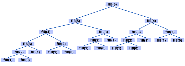
Here’s an algorithm (non-parallel) for computing Fibonacci numbers based on the above definition:

algorithm FIB(n):
    // INPUT
    //    n = a non-negative integer
    // OUTPUT
    //    The nth Fibonacci number

    if n <= 1:
        return n
    else:
        x <- FIB(n-1)
        y <- FIB(n-2)
        return x + y

Here’s the recursion tree of the algorithm cited above:

Let’s see what improvement we can get by computing the two recursive calls in parallel using the concurrency keywords:

algorithm P-FIB(n):
    // INPUT
    //    n = non-negative integer
    // OUTPUT
    //    The nth Fibonacci number computed in parallel

    if n <= 1:
        return n
    else:
        x <- spawn P-FIB(n-1) // parallel execution
        y <- spawn P-FIB(n-2) // parallel execution
        sync // wait for the results x and y
        return x + y

4. Modeling Dynamic Multithreading

Let’s now look at a formal model for describing parallel computations.

4.1. Computation DAG

A computation DAG (directed acyclic graph) will be used to model a multithreaded computation ${G = (V, E)}$ :

Vertices: vertices ( ${V}$ ) in the graph represent the instructions. To simplify, let’s think of each vertex as a strand (sequence of instructions containing no parallel control, such as sync, spawn, parallel, return from spawn)
Edges: edges ( ${E}$ ) represent the dependencies between strands or instructions. An edge ${(u,v)}$ in ( ${E}$ ) indicates that instruction ( ${u}$ ) must be executed before instruction ( ${v}$ )

If there’s an edge between thread (a strand of maximal length will be called a thread) ${u}$ and ${v}$ they are logically in series; otherwise, they are logically parallel.

4.2. Edge Classification

Here’s a categorization of the edges:

Continuation edge ${(u,v)}$ : connects a thread ${u}$ to its successor ${v}$ within the same procedure instance
Spawn edge ${(u,v)}$ : ${(u,v)}$ is called a spawn edge when a thread ${u}$ spawns a new thread ${v}$ in parallel
Return edge ${(v,x)}$ : when a thread ${v}$ returns to its calling process and ${x}$ is the thread following the parallel control, the graph includes the return edge ${(v,x)}$

4.3. Visualization of the Model

Before moving forward to the model for the computation DAG, let’s take a look at the parallel algorithm to compute Fibonacci numbers using threads:

algorithm P-FIB(n):
    // INPUT
    //    n = non-negative integer
    // OUTPUT
    //    The nth Fibonacci number, with thread annotations for clarity

    if n <= 1:
        return n  // Thread A
    else:
        x <- spawn P-FIB(n-1) // Thread A continues
        y <- spawn P-FIB(n-2) // Thread B
        sync // wait for results
        return x + y  // Thread C combines results

Here’s the model for the computation DAG for P-FIB( ${4}$ ):

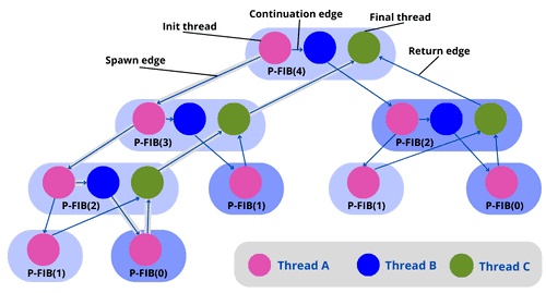
As we can see in the figure above, the purple thread in the block number ${4}$ spawns another purple thread in the block number ${3}$ . Then the number ${3}$ points to the purple thread in the block number ${2}$ . The number ${2}$ points to the purple thread in the block number ${2}$ . Then we point to the green thread in the block number ${2}$ using the return edge. We continue pointing to the green thread in block number ${3}$ and ${4}$ until we reach the final thread.

5. Measuring Dynamic Multithreading

Let’s walk through some measures and observations the characterizes dynamic multithreading.

5.1. Work

The work of a multithreaded computation is the total time required to execute the entire computation on one processor. So, the work represents the sum of the time taken by each thread.

An ideal parallel computer with ${P}$ processors can perform up to ${P}$ units of work in a one-time step. In other words, it can do up to ${P \times T_{P}}$ work in ${T_{P}}$ time ( ${T_{P}}$ is the running time of an algorithm on ${P}$ processors). Since the total work is ${T_{1}}$ , ${P \times T_{P} \geq T_{1}}$ . Hence, the work law is $\boldsymbol{T_{P} \geq \frac{ T_{1}}{P}}$ .

5.2. Span

The span is the longest time it takes to execute threads along any path of the computational DAG.

An ideal parallel computer with ${P}$ processors cannot run faster than a machine with an infinite number of processors. A computer with an infinite number of processors, on the other hand, can imitate a ${P}$ processor machine by employing only ${P}$ of its processors. Therefore, $\boldsymbol{T_{P} \geq T}$ , which is known as the span law.

5.3. Speedup and Parallelism

The speedup of a computation on ${P}$ processors is ${\frac{T_{1}}{T_{P}}$ . So, this ratio defines how much speedup we get with the ${P}$ processor as compared to one. Using the work law ( ${T_{P} \geq \frac{ T_{1}}{P} \text{ so, } \frac{ T_{1}}{T_{P}} \leq {P} }$ ), we can conclude that an ideal parallel computer cannot have any more speedup than the number of processors.

The parallelism of a multithreaded computation is ${\frac{T_{1}}{T_{\infty}}$ . So, this ratio means the average amount of work that can be performed for each step of parallel execution time.

5.4. Slackness

The parallel slackness of a multithreaded calculation performed on an ideal parallel computer with ${P}$ processors is defined as the parallelism by ${P}$ ratio:

${Slackness = \frac{(\frac{T_{1}}{T_{\infty}})}{P}}$

5.5. Performance Measure Example

Let’s use the Fibonacci example (P-FIB( ${4}$ )). In the graph below, we use ${17}$ threads ( ${17}$ vertices). As we can see, there are ${8}$ threads on the longest path (red line in the graph).

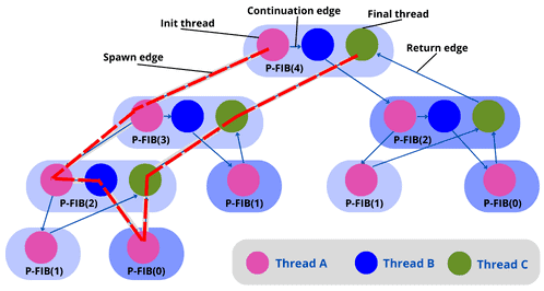
Example of Multithreaded Algorithm (Fibonacci DAG)

Let’s assume the unit time for each thread:

Work: ${17}$ time units
Span: ${8}$ time units

Let’s now take a look at the work and span of the Fibonacci computation (using the parallel algorithm above of P-FIB( ${n}$ )) to compute the parallelism:

The work ${T_{1}}$ is simple since it computes the execution time of the serialized algorithm:

${T_{1} = \theta((\frac{1+\sqrt{5}}{2})^n )}$

We know that the span ${T_{\infty}}$ is the longest path in the computational DAG. So, P-FIB( ${n}$ ) spawns: P-FIB( ${n-1}$ ) and P-FIB( ${n-2}$ ). Then, here’s the longest path ${T_{\infty}}$ :

${T_{\infty}(n) = max( T_{\infty}(n-1) , T_{\infty}(n-2) ) + \theta(1) = T_{\infty}(n-1) + \theta(1) \text{ which yields } T_{\infty}(n) = \theta(n)}$

Here’s the parallelism of the P-FIB computation:

${\frac{T_{1}(n)}{T_{\infty}(n)} = \theta(\frac{(\frac{1+\sqrt{5}}{2})^n )}{n}) \text{ which grows dramatically as n gets large }}$

6. Additional Examples

Let’s now use an example to understand the multithreading algorithm and its operations (parallel, spawn, sync).

6.1. Multithreaded Matrix Multiplication Algorithm

Here’s an algorithm for multithreaded matrix multiplication, using the ${T_{1}(n) = \theta(n^3)}$ algorithm:

algorithm P-Matrix-Multiply(A, B):
    // INPUT
    //    A, B = square matrices of size n x n
    // OUTPUT
    //    C = the product of A and B, computed in parallel
    
    n <- the number of rows in A
    
    C <- initialize an empty n x n matrix
    parallel for i <- 1 to n:
        parallel for j <- 1 to n:
            c[i, j] <- 0
            for k <- 1 to n:
                c[i, j] <- c[i, j] + a[i, k] * b[k, j]
    return C

In this algorithm, the longest path is when spawning the outer and inner parallel loop executions, and then the ${n}$ executions of the innermost for loop. So, the span of this algorithm is ${T_{\infty}(n) = \theta(n)}$ . Hence, the parallelism is ${ \frac{T_{1}(n)}{T_{\infty}(n)} = \frac{\theta(n^3)}{\theta(n)} = \theta(n^2)}$ .

6.2. Multithreaded Merge Sort Algorithm

We employ divide-and-conquer algorithms for parallelism because they divide the problem into independent subproblems that can be addressed individually. Let’s take a look at merge sort:

algorithm Merge-Sort(a, p, r):
    // INPUT
    //    a = array to sort
    //    p = starting index
    //    r = ending index
    // OUTPUT
    //    Array a sorted in place from indices p to r

    if p < r:
        q <- (p + r) / 2
        spawn Merge-Sort(a, p, q)
        Merge-Sort(a, q+1, r)
        sync // wait for parallel processes to complete
        Merge(a, p, q, r)

As we can see, the dividing is in the main procedure Merge-Sort, then we parallelize it by using spawn on the first recursive call. Merge remains a serial algorithm, so its work and span are ${\theta(n)}$ as before.

Here’s the recurrence for the work ${T_{1}(n)}$ of Merge-Sort (it’s the same as the serial version):

${T_{1}(n) = 2 \times T_{1}(\frac{n}{2}) + \theta(n) = \theta(n \times \log(n))}$

The recurrence for the span ${T_{\infty}(n)}$ of Merge-Sort is based on the fact that the recursive calls run in parallel:

${T_{\infty}(n) = T_{\infty}(\frac{n}{2}) + \theta(n) = \theta(n)}$

Here’s the parallelism:

${\frac{T_{1}(n)}{T_{\infty}(n)} = \theta(\frac{n \times \log(n)}{n}) = \theta(\log(n))}$

As we can see, this is low parallelism, which means that even with massive input, having hundreds of processors would not be beneficial. So, to increase the parallelism, we can speed up the serial Merge.

7. Application of Multithreading

Here are some applications of using multithreading:

Simultaneous access to a dataset
Web server handling new connections while still listening on a port
Encrypting files on a background thread, while an application runs on the main thread

8. Conclusion

In this tutorial, we’ve discussed the basic concept of multithreaded algorithms using an example to unlock its mechanism. We’ve also gone over the directed acyclic graph (DAG).

Learn Java Collections

Learn Spring

Learn Maven

View All Courses

Core Concepts

Operating Systems

Neural Networks

Graph Theory

Latex

Full Archive

About Baeldung